Turbulence transports momentum, heat, and species through nonlinear interactions among eddies of many sizes. Our laboratory uses direct numerical simulation (DNS) to resolve these scales, investigate the fundamental structure of turbulent flows, and construct reference data for engineering models.

DNS provides time-resolved fields of velocity, pressure, and temperature. These data support physical analysis and provide labelled data for sub-grid-scale (SGS) models in large-eddy simulation (LES). We connect high-fidelity simulation with AI modelling to predict complex flows at a practical computational cost.

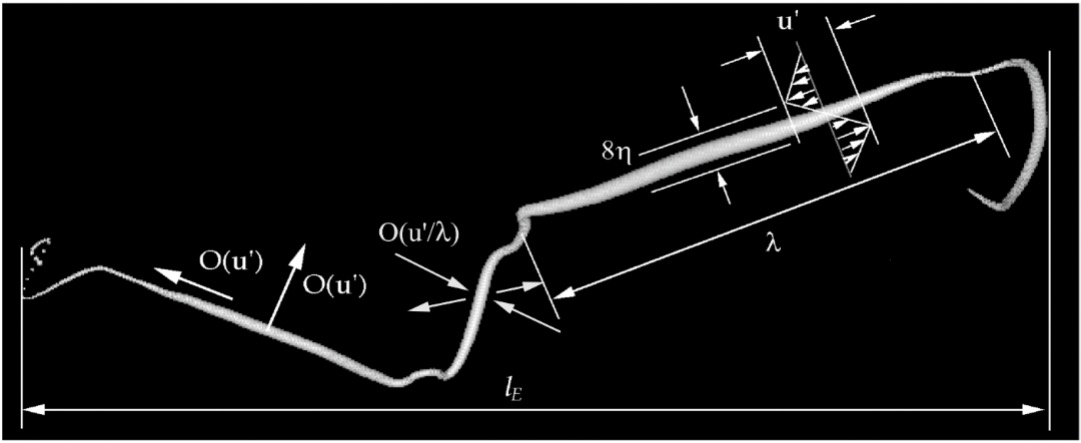
DNS solves the governing equations on a grid without averaging the turbulence or replacing small eddies with empirical closures. It must resolve the largest flow structures as well as the small scales where viscosity dissipates energy. The computational cost is high, but the resulting data retain the detailed physics without SGS-model assumptions.

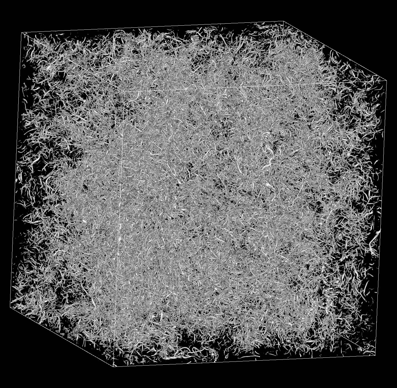
We perform DNS of homogeneous isotropic turbulence, channel flow, and mixing layers. By varying boundary conditions, shear, and Reynolds number, we examine structures shared across flows and the changes introduced by walls and mean shear.

Unlike homogeneous turbulence, practical flows involve walls, curved surfaces, and differences in flow speed. These conditions change the size, direction, and movement of vortices, and therefore affect drag and the transport of heat and matter. DNS adds these conditions one at a time to identify where and why turbulence becomes stronger.

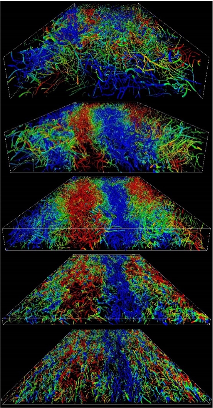
In wall-shear turbulence, velocity changes rapidly close to the wall. The small vortices produced by this change affect friction and heat transfer. This matters for reducing drag on vehicles and aircraft, for internal pipe flow, and for devices that transport heat efficiently.

DNS follows these structures over time rather than showing only an average flow.

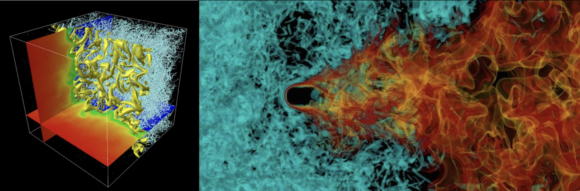
Free-shear turbulence develops where two streams with different velocities meet. Vortices at their boundary entrain surrounding fluid and mix the streams. This process matters for fuel-air mixing, exhaust dispersion, and the transport of heat and species. Studying it reveals how vortices grow and transport heat and matter.

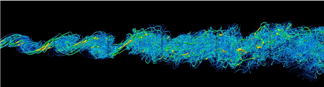
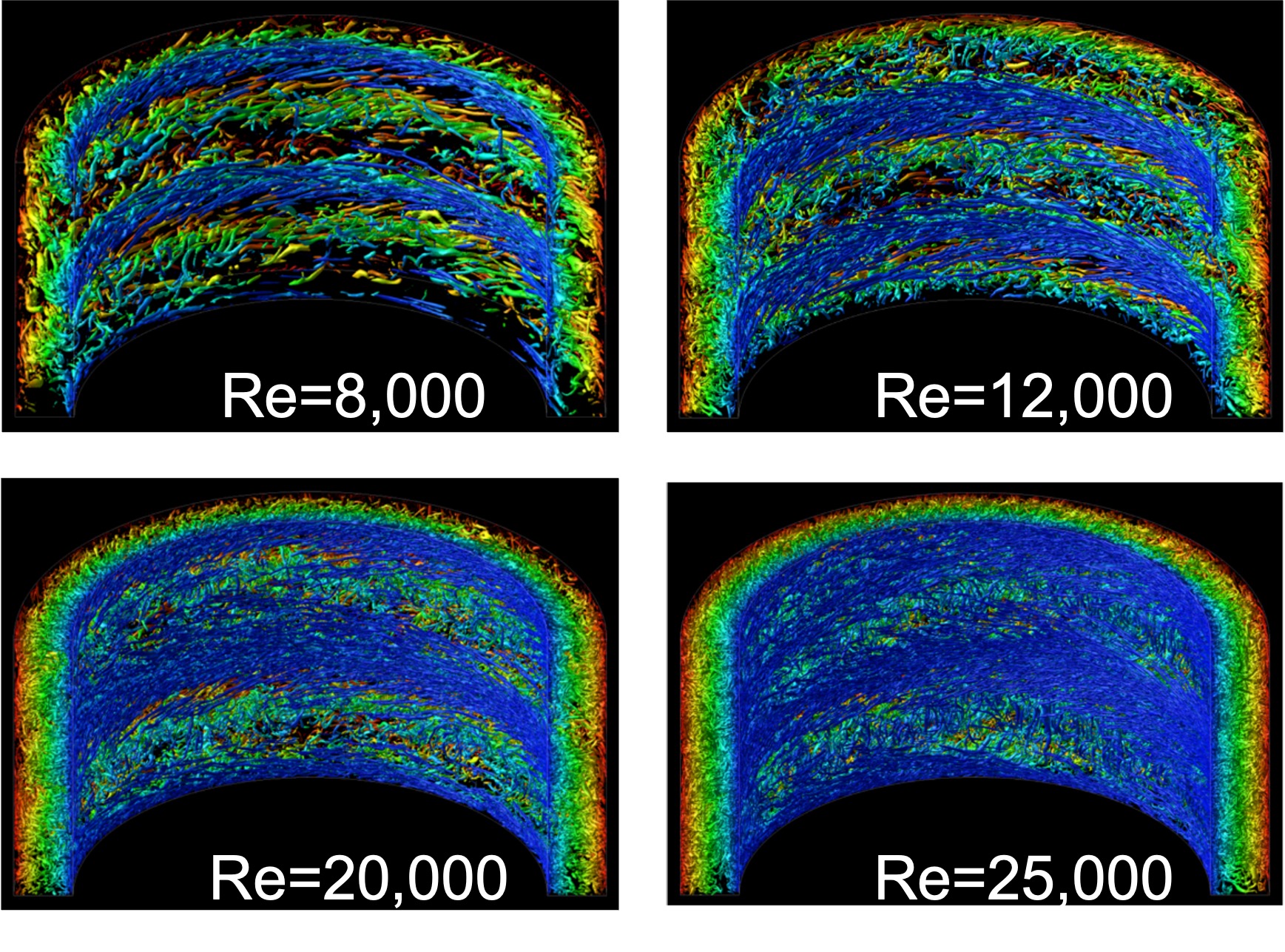
Even in the same annular channel, vortices change in number and detail as the flow speed increases. Comparing Reynolds numbers tests whether insight from one condition still applies to another, which is essential when applying research results to real equipment.

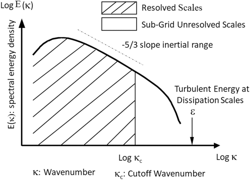
LES resolves large eddies while representing motions smaller than the grid with an SGS model. The unresolved motions beyond the cut-off wavenumber contribute to turbulent energy transfer and dissipation, so they must be represented appropriately.

Conventional eddy-viscosity and similarity models can lose accuracy when the flow type, wall distance, or grid width changes. DNS makes the correspondence between the resolved field and the target SGS stress explicit.

DNS records the fine detail of turbulence much like a high-resolution movie. We use this information to teach AI how small, unresolved eddies affect the flow, so that simulations can make useful estimates with less computational effort.

Preparing data for AI

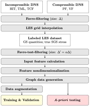
We first organise the detailed DNS results into a form used by practical simulations such as LES. The resulting dataset lets the AI learn how the surrounding flow relates to the effect of eddies that are too small to calculate directly.

Learning from different turbulent flows

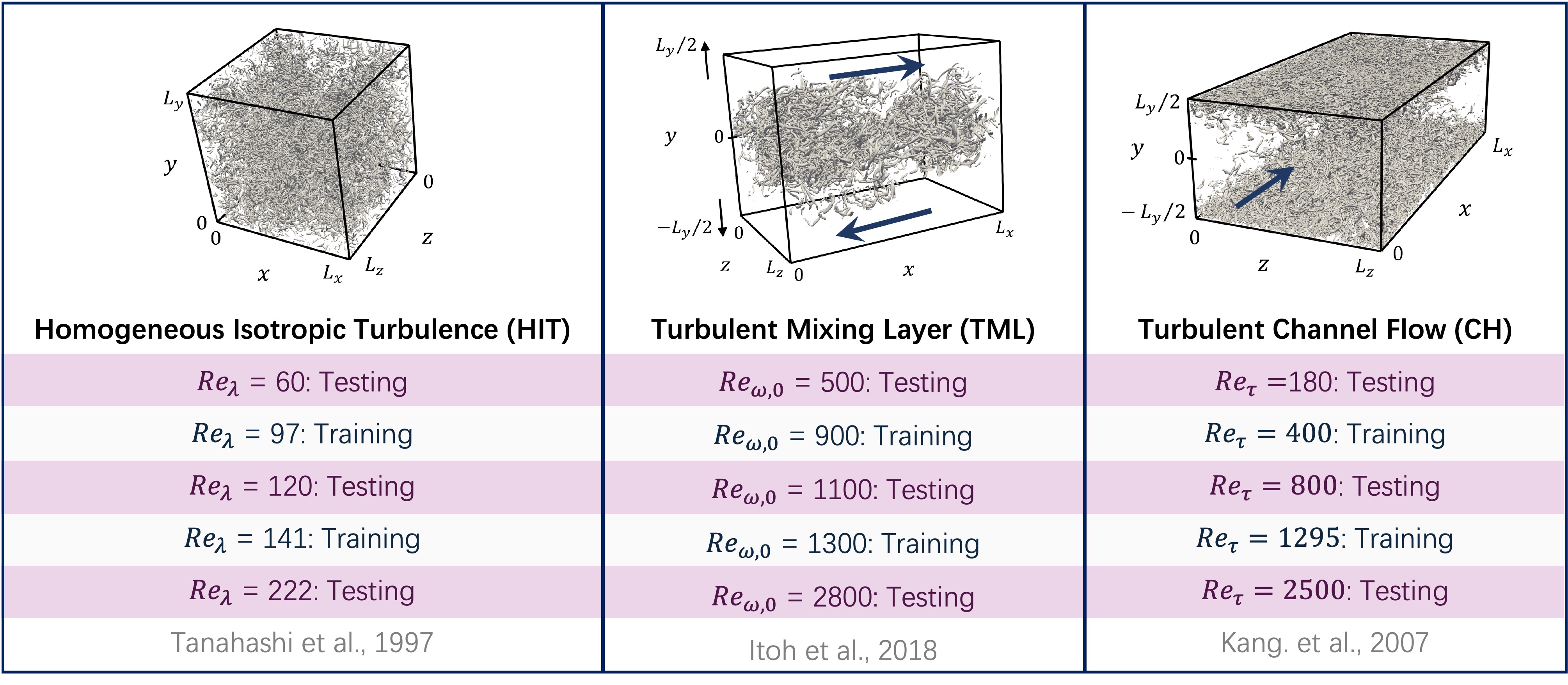
An AI trained on one flow alone can learn that particular condition too closely. We therefore use DNS data for freely evolving turbulence, mixing layers, and wall-bounded flows, then test whether the model remains useful under different conditions.

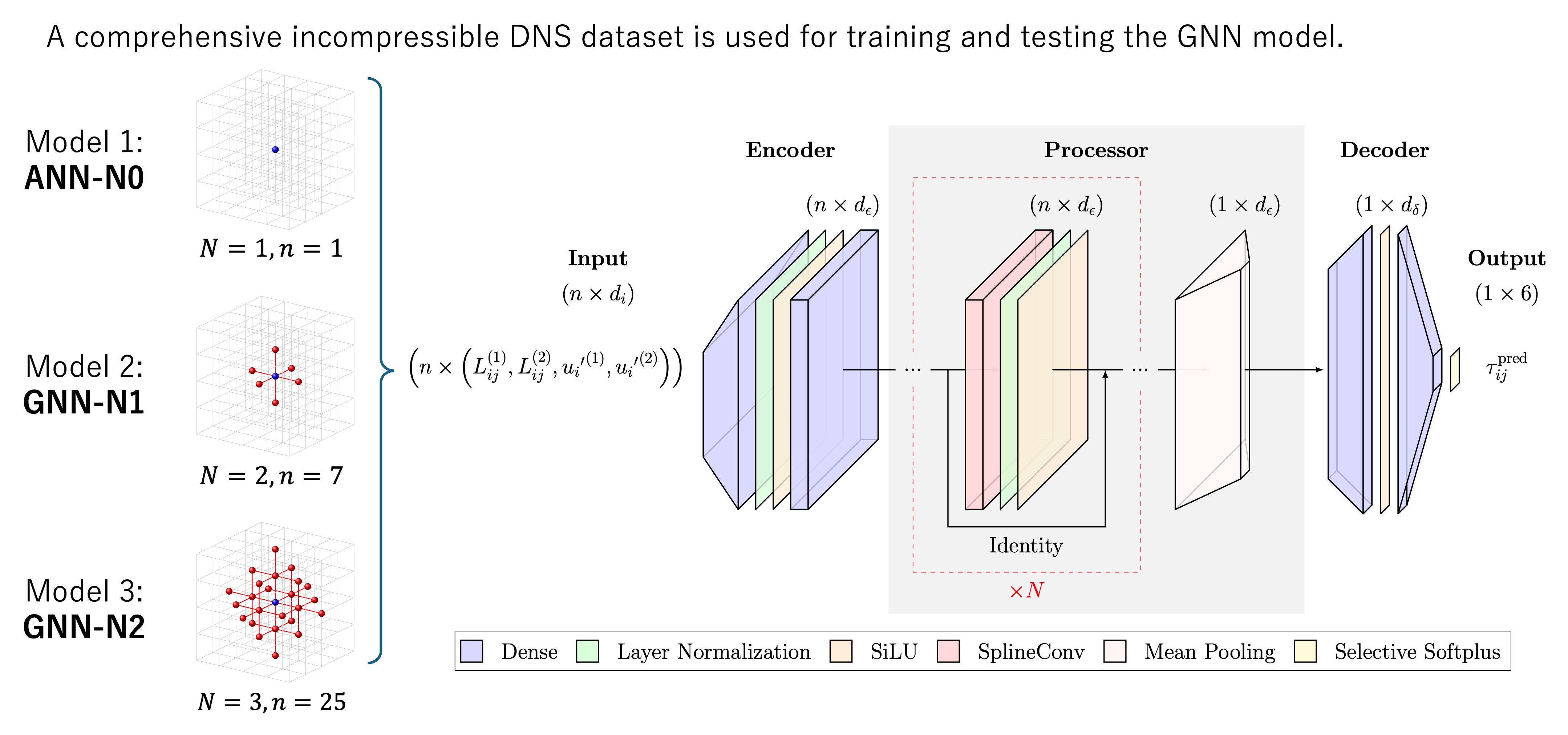
Using GNNs to look at the surrounding flow

A conventional AI model mainly uses information at one calculation point. A GNN also considers the relationship between that point and nearby points. This resembles using the surrounding area of a photograph to understand what is happening in one small part of it.

ANN-N0 is a comparison model that looks only at the centre point. GNN-N1 and GNN-N2 use progressively wider neighbourhoods. DNS data lets us examine how much surrounding information improves prediction.

We test whether the model can still make useful predictions for conditions excluded from training. The figure compares ANN and GNN results for three types of turbulence. GNNs, which use surrounding information, show stable predictions in many cases.

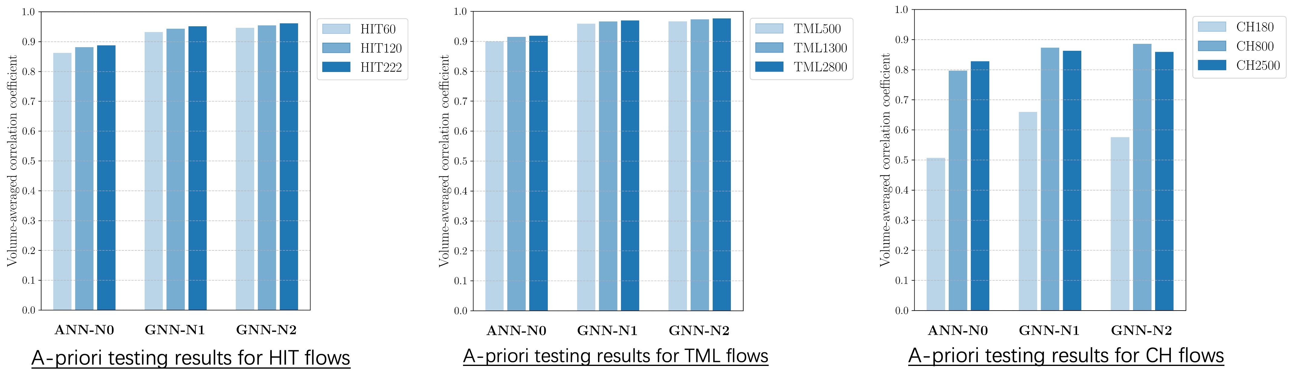
These checks help distinguish genuine learning of flow behaviour from simple memorisation of training data. In the future, this approach can support faster and more reliable design simulations for engines, combustors, and other engineering systems.

DNS remains too computationally expensive for most full-scale design calculations. It nevertheless provides the basis for testing turbulence-model assumptions and defining the physical quantities that AI should learn. We combine DNS, physics-based statistical analysis, and machine learning to improve both accuracy and computational efficiency.

Figures are based on the presentation “Direct Numerical Simulation of Turbulence and AI Modelling”.